Linear Quadratic Problem
In this blog, we introduce the recursive method for solving the following LQR problem:
\[\begin{aligned} \min_{\bar{x}, \bar{u}} \quad &\sum_{k=0}^{N-1} \begin{bmatrix} q_k \\ r_k \end{bmatrix}^\top \begin{bmatrix} x_k \\ u_k \end{bmatrix} + \frac{1}{2} \begin{bmatrix} x_k \\ u_k \end{bmatrix}^\top \begin{bmatrix} Q_k & S_k^\top \\ S_k & R_k \end{bmatrix} \begin{bmatrix} x_k \\ u_k \end{bmatrix} \\ &\quad\quad + p_N^\top x_N + \frac{1}{2} x_N^T P_N x_N \\ \text{s.t.}\quad & x_{k+1} = A_k x_k + B_k u_k + c_k,\; k = 0, \dots, N-1, \end{aligned}\]where $\bar{x} := \{ x_1, \dots, x_N \}$ and $\bar{u} := \{ u_0, \dots, u_{N-1} \}$. We consider the LQR problem as a quadratic program with equality constraints. The corresponding Lagrangian is then expresed as
\[\begin{aligned} \mathcal{L} (\bar{x}, \bar{u}, \bar{\lambda}) &= \sum_{k=0}^{N-1} \Bigg( \begin{bmatrix} q_k \\ r_k \end{bmatrix}^\top \begin{bmatrix} x_k \\ u_k \end{bmatrix} + \frac{1}{2} \begin{bmatrix} x_k \\ u_k \end{bmatrix}^\top \begin{bmatrix} Q_k & S_k^\top \\ S_k & R_k \end{bmatrix} \begin{bmatrix} x_k \\ u_k \end{bmatrix} + \lambda_{k+1}^\top \left(A_k x_k + B_k u_k + c_k - x_{k+1} \right) \Bigg) \\ &\quad\quad\quad + p_N^\top x_N + \frac{1}{2} x_N^T P_N x_N, \end{aligned}\]where $\bar{\lambda} = (\lambda_1, \cdots, \lambda_N)$ is a vector of Lagrange multipliers. The KKT conditions are derived as
\[\begin{aligned} \frac{\partial \mathcal{L}}{\partial \bar{x}} = 0,\; \frac{\partial \mathcal{L}}{\partial \bar{u}} = 0,\; \frac{\partial \mathcal{L}}{\partial \bar{\lambda}} = 0. \end{aligned}\]For $k = 0$,
\[\begin{aligned} 0 &= r_0 + R_0 u_0 + S_0 x_0 + B_0^\top \lambda_{1}. \end{aligned}\]For $0 < k <= N-1$,
\[\begin{aligned} 0 &= q_k + Q_k x_k + S_k^\top u_k + A_k^\top \lambda_{k+1} - \lambda_k , \\ 0 &= r_k + R_k u_k + S_k x_k + B_k^\top \lambda_{k+1}, \\ 0 &= A_{k-1} x_{k-1} + B_{k-1} u_{k-1} + c_{k-1} - x_k. \end{aligned}\]For $k = N$,
\[\begin{aligned} 0 &= p_N + P_N x_N - \lambda_N , \\ 0 &= A_{N-1} x_{N-1} + B_{N-1} u_{N-1} + c_{N-1} - x_N. \end{aligned}\]The corresponding KKT system $(N = 3)$ is then
\[\begin{equation*} \left[ \begin{array}{ccccccccc} R_0 & B_0^\top \\ B_0 & & -I\\ \hline & -I & Q_1 & S_1^\top & A_1^\top \\ & & S_1 & R_1 & B_1^\top \\ & & A_1 & B_1 & & -I \\ \hline & & & & -I & Q_2 & S_2^\top & A_2^\top \\ & & & & & S_2 & R_2 & B_2^\top \\ & & & & & A_2 & B_2 & & -I \\ \hline & & & & & & & -I & P_3 \end{array} \right] \left[ \begin{array}{c} u_0 \\ \lambda_1 \\ \hline x_1 \\ u_1 \\ \lambda_2 \\ \hline x_2 \\ u_2 \\ \lambda_3 \\ \hline x_3 \end{array} \right] = \left[ \begin{array}{c} -r_0 - S_0 x_0 \\ -A_0 x_0 - c_0 \\ \hline -q_1 \\ -r_1 \\ -c_1 \\ \hline -q_2 \\ -r_2 \\ -c_2 \\ \hline -p_3 \end{array} \right] \end{equation*}.\]Next, we recursively factorize the KKT matrix, starting from the last two stages:
\[\begin{equation*} \left[ \begin{array}{ccccccccc} -I & Q_{N-1} & S_{N-1}^\top & A_{N-1}^\top \\ & S_{N-1} & R_{N-1} & B_{N-1}^\top \\ & A_{N-1} & B_{N-1} & & -I \\ \hline & & & -I & P_N \end{array} \right] \left[ \begin{array}{c} \lambda_{N-1} \\ \hline x_{N-1} \\ u_{N-1} \\ \lambda_{N} \\ \hline x_N \end{array} \right] = \left[ \begin{array}{c} -q_{N-1} \\ -r_{N-1} \\ -c_{N-1} \\ \hline -p_N \end{array} \right] \end{equation*}.\]By adding the 4th row to the 3rd row multiplied by $P_N$, we can eliminate the 4th row and obtain
\[\begin{equation*} \left[ \begin{array}{ccccccccc} -I & Q_{N-1} & S_{N-1}^\top & A_{N-1}^\top \\ & S_{N-1} & R_{N-1} & B_{N-1}^\top \\ & P_N A_{N-1} & P_N B_{N-1} & -I \end{array} \right] \left[ \begin{array}{c} \lambda_{N-1} \\ \hline x_{N-1} \\ u_{N-1} \\ \lambda_{N} \end{array} \right] = \left[ \begin{array}{c} -q_{N-1} \\ -r_{N-1} \\ -P_N c_{N-1} - p_N \end{array} \right] \end{equation*}.\]To eliminate the 3rd row, we add it multiplied by $\textcolor{red}{A_{N-1}^\top}$ to the 1st row and add it multiplied by $\textcolor{blue}{B_{N-1}^\top}$ to the 2nd row, resulting in
\[\begin{equation*} \left[ \begin{array}{ccccccccc} -I & Q_{N-1} + \textcolor{red}{A_{N-1}^\top} P_N A_{N-1} & S_{N-1}^\top + \textcolor{red}{A_{N-1}^\top} P_N B_{N-1} \\ & S_{N-1} + \textcolor{blue}{B_{N-1}^\top} P_N A_{N-1} & R_{N-1} + \textcolor{blue}{B_{N-1}^\top} P_N B_{N-1} \\ \end{array} \right] \left[ \begin{array}{c} \lambda_{N-1} \\ \hline x_{N-1} \\ u_{N-1} \end{array} \right] = \left[ \begin{array}{c} -q_{N-1} - A_{N-1}^\top (P_N c_{N-1} + p_N) \\ -r_{N-1} - B_{N-1}^\top (P_N c_{N-1} + p_N) \end{array} \right] \end{equation*}.\]For notational simplicity, we use
\[\begin{aligned} Q_{xx,k} &= Q_{k} + A_k^\top P_{k+1}A_k\\ Q_{uu,k} &= R_{k} + B_k^\top P_{k+1}B_k\\ Q_{ux,k} &= S_{k} + B_k^\top P_{k+1}A_k \\ Q_{x,k} &= q_k + A_k^\top \left( P_{k+1} c_k + p_{k+1} \right)\\ Q_{u,k} &= r_k + B_k^\top \left( P_{k+1} c_k + p_{k+1} \right). \end{aligned}\]We then represent $u_{N-1}$ in terms of $x_{N-1}$
\[\begin{aligned} Q_{ux, N-1} x_{N-1} + Q_{uu, N-1} u_{N-1} &= - Q_{u, N-1} \\ u_{N-1} &= - Q_{uu, N-1}^{-1} Q_{ux, N-1} x_{N-1} - Q_{uu, N-1}^{-1} Q_{u, N-1} \\ &:= K_{N-1} x_{N-1} + d_{N-1}. \end{aligned}\]We also have
\[\begin{aligned} -\lambda_{N-1} + Q_{xx, N-1} x_{N-1} + Q_{ux, N-1}^\top u_{N-1} &= - Q_{x, N-1} \\ -\lambda_{N-1} + Q_{xx, N-1} x_{N-1} + Q_{ux, N-1}^\top (-Q_{uu, N-1}^{-1} Q_{ux, N-1} x_{N-1} - Q_{uu, N-1}^{-1} Q_{u, N-1}) &= -Q_{x, N-1} \end{aligned}\] \[\begin{aligned} \lambda_{N-1} &= \left( Q_{xx, N-1} - Q_{ux, N-1}^\top Q_{uu, N-1}^{-1} Q_{ux, N-1} \right) x_{N-1} + Q_{x, N-1} - Q_{ux, N-1}^\top Q_{uu, N-1}^{-1} Q_{u, N-1} \\ &:= P_{N-1} x_{N-1} + p_{N-1}. \end{aligned}\]This indicates the relation between $\lambda_k$ and $x_k$, and it is not difficult to derive the submatrix to be factorized at stage $k$
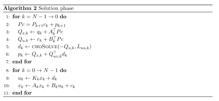
\[\begin{equation*} \left[ \begin{array}{ccccccccc} -I & Q_{k} & S_{k}^\top & A_{k}^\top \\ & S_{k} & R_{k} & B_{k}^\top \\ & A_{k} & B_{k} & & -I \\ \hline & & & -I & P_{k+1} \end{array} \right] \left[ \begin{array}{c} \lambda_{k} \\ \hline x_{k} \\ u_{k} \\ \lambda_{k+1} \\ \hline x_{k+1} \end{array} \right] = \left[ \begin{array}{c} -q_{k} \\ -r_{k} \\ -c_{k} \\ \hline -p_{k+1} \end{array} \right] \end{equation*}.\]We can repeat the same procedure as above to factorize this submatrix until the initial stage. After the factorization phase, we use the computed matrices $K_k$ and $d_k$ to recover the optimal state and input trajectories. This is called the solution phase. The descriptions of the two algorithms are shown below.
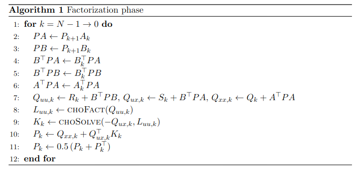
Note that Line 11 in Algorithm 1 can improve the numerical stability. The methods $\texttt{choFact}$ and $\texttt{choSolve}$ compute the Cholesky decomposition and solve the linear system using the Cholesky factorization, respectively.
Before proceeding with complexity analysis, we introduce the concept of the FLOP (Floating-Point Operation), which refers to a single operation involving floating-point numbers, such as:
- addition: $a + b$
- subtraction: $a - b$
- multiplication: $a b$
- division: $a/b$
We often use flop counts to roughly estimate the computation time of a numerical method. Below, we present the flop counts relevant to this tutorial. For further details, please refer to Appendix C of the book by Boyd and Vandenberghe.
| Operation | FLOP Count (Approx.) | Notes |
|---|---|---|
| Dot product of two $n$-vectors | $2n$ | $n$ mults + $n-1$ adds |
| Matrix-vector multiplication $A \in \mathbb{R}^{m \times n}, b \in \mathbb{R}^{n}$ | $2mn$ | Each row requires a dot product |
| Matrix-matrix multiplication $A \in \mathbb{R}^{m \times k}, B \in \mathbb{R}^{k \times n}$ | $2mkn$ | Without parallelization |
| Solving triangular system (e.g., forward/back substitution) | $n^2$ | For $n \times n$ lower or upper triangular matrix |
| Cholesky factorization $A = LL^\top$, $A \in \mathbb{R}^{n \times n}$ | $\frac{1}{3}n^3$ | For dense matrices |
| Cholesky solve $b \in \mathbb{R}^{n \times p}, Ly = b, L^\top x = y$ | $2n^2p$ |
We now separately count the number of flops required for the factorization and solution phases. In the factorization phase, we consider only the cubic terms, while in the solution phase, we focus solely on the quadratic terms.
Factorization phase
| Expression | FLOP Count (Approx.) |
|---|---|
| $PA \leftarrow P_{k+1} A_k$ | $2n_x^3$ |
| $PB \leftarrow P_{k+1} B_k$ | $2n_x^2 n_u$ |
| $B^\top PA \leftarrow B_k^\top PA$ | $2n_x^2 n_u$ |
| $B^\top PB \leftarrow B_k^\top PB$ | $2n_x n_u^2$ |
| $A^\top PA \leftarrow A_k^\top PA$ | $2n_x^3$ |
| $L_{uu, k} \leftarrow \texttt{choFact}(Q_{uu, k})$ | $\frac{1}{3}n_u^3$ |
| $K_k \leftarrow \texttt{choSolve}(-Q_{ux, k}, L_{uu, k})$ | $2n_x n_u^2$ |
| $P_k \leftarrow Q_{xx, k} + Q_{ux, k}^\top \cdot K_k$ | $2n_x^2 n_u$ |
Total flop counts:
\[N (4n_x^3 + 6n_x^2 n_u + 4n_x n_u^2 + \frac{1}{3}n_u^3)\]Solution phase
| Expression | FLOP Count (Approx.) |
|---|---|
| $Pc = P_{k+1}c_k + p_{k+1}$ | $2n_x^2$ |
| $Q_{x, k} \leftarrow q_k + A_k^\top Pc$ | $2n_x^2$ |
| $Q_{u, k} \leftarrow r_k + B_k^\top Pc$ | $2n_x n_u$ |
| $d_k \leftarrow \texttt{choSolve}(-Q_{u, k}, L_{uu, k})$ | $2n_u^2$ |
| $p_k \leftarrow Q_{x, k} + Q_{ux, k}^\top d_k$ | $2n_x n_u$ |
| $u_k \leftarrow K_k x_k + d_k $ | $2n_x n_u$ |
| $x_k \leftarrow A_k x_k + B_k u_k + c_k$ | $2n_x^2 + 2n_x n_u$ |
Total flop counts:
\[N (6 n_x^2 + 8 n_x n_u + 2 n_u^2)\]Efficient Riccati Recursion
In this section, we improve the efficiency of the Riccati recursion. First, we introduce some useful matrix operations.
| Operation | FLOP Count (Approx.) |
|---|---|
| Triangular Matrix-matrix multiplication (trmm) $A \in \mathbb{R}^{m \times m} (\text{triangular matrix}), B \in \mathbb{R}^{m \times n}$ | $m^2n$ |
| Symmetric Rank-k Update (syrk) $A \in \mathbb{R}^{m \times n},\; A A^\top$ | $m^2 n$ |
The square-root Riccati recursion is proposed in [1]. The key idea is to carry out the recursion in terms of the Cholesky factor $\mathcal{L}_k$ rather than $P_k$. The algorithm is provided below, along with the flop counts.
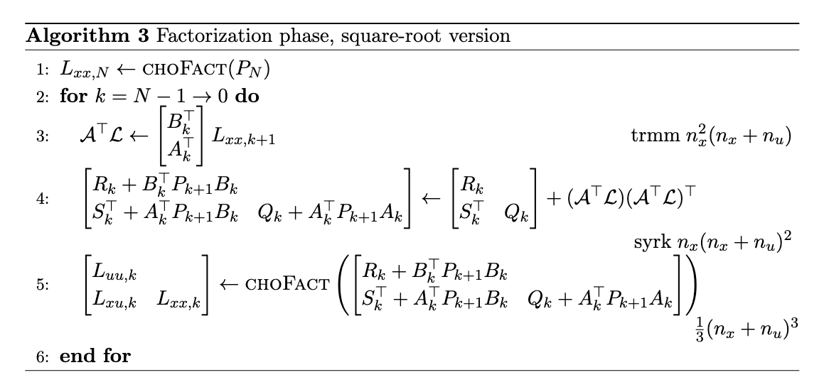
The total flop counts are
\[N \left(\frac{7}{3} n_x^3 + 4 n_x^2 n_u + 2 n_x n_u^2 + \frac{1}{3} n_u^3 \right).\]Let us have a close look at Line 5.
\[\begin{bmatrix} L_{uu, k} \\ L_{xu, k} & L_{xx, k} \end{bmatrix} \begin{bmatrix} L_{uu, k} \\ L_{xu, k} & L_{xx, k} \end{bmatrix}^\top = \begin{bmatrix} L_{uu, k} L_{uu, k}^\top & L_{uu, k} L_{xu, k}^\top \\ L_{xu, k} L_{uu, k}^\top & L_{xu, k} L_{xu, k}^\top + L_{xx, k} L_{xx, k}^\top \end{bmatrix} = \begin{bmatrix} R_k + B_k^\top P_{k+1} B_k \\ S_k^\top + A_k^\top P_{k+1} B_k & Q_k + A_k^\top P_{k+1} A_k \end{bmatrix}\] \[\begin{aligned} L_{uu, k} &= \texttt{choFact} (R_k + B_k^\top P_{k+1} B_k) \\ L_{xu, k} &= (S_k^\top + A_k^\top P_{k+1} B_k) L_{uu, k}^{-\top} \\ L_{xx, k} &= \texttt{choFact} (Q_k + A_k^\top P_{k+1} A_k - L_{xu, k} L_{xu, k}^\top) \end{aligned}\] \[\begin{aligned} Q_k + A_k^\top P_{k+1} A_k - L_{xu, k} L_{xu, k}^\top &= Q_k + A_k^\top P_{k+1} A_k - (S_k^\top + A_k^\top P_{k+1} B_k) L_{uu, k}^{-\top} L_{uu, k}^{-1} (S_k^\top + A_k^\top P_{k+1} B_k)^\top \\ &:= Q_{xx, k} - Q_{ux, k}^\top Q_{uu, k}^{-1} Q_{ux, k} \\ &:= Q_{xx, k} + Q_{ux, k}^\top K_k \end{aligned}\]Finally, refer to the repository for implementation details.
References
- Efficient implementation of the Riccati recursion for solving linear-quadratic control problemsIn 2013 IEEE International Conference on Control Applications (CCA) , 2013