Contact Dynamics: Introduction

Simulating multibody systems with frictional contact is crucial in robotics, particularly for training robotic systems. This blog introduces some fundamental concepts of contact modeling. Let’s consider the contact between the point foot of a quadruped and the ground. We define the gap function $\phi(q)$ as the signed distance between the point foot and the ground, where $q$ represents the generalized positions.

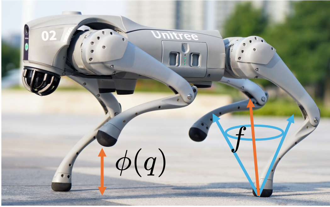
The contact force $f$, expressed in the local contact frame, consists of the tangential component $f_T$ and the normal component $f_N$. The magnitude and direction of the contact force are not arbitrary. As you may have heard, the contact force should lie within the so-called friction cone. One of our main goals is to identify the constraints related to this force, and we will dive into those details later. But for now, let’s step back and look at the bigger picture — what exactly are we trying to compute when simulating a single time step? We assume that you are familiar with the following equation of motion:

\[M (q)\dot{v} = \tau - h(q, v) + J(q)^\top \boldsymbol{f},\]

where $v$ is the generalized velocity, $M(q)$ denotes the joint space inertia matrix, $h(q, v)$ accounts for the centrifugal, Coriolis, and gravitational effects, and $\tau$ is the actuation torque. The collection of contact forces is denoted as $\boldsymbol{f} \in \mathbb{R}^{3 N_c}$, where $N_c$ is the number of contacts that the robot makes at the current time instance. $J(q)$ represents the Jacobian, which maps the generalized velocity to the collection of contact velocities expressed in the local contact frames. To discretize the system, we adopt the semi-implicit Euler integration scheme:

\[M(q_t)(v_{t+1} - v_t) = \Delta t\left(\tau_t - h(q_t, v_t)\right) + J(q_t)^\top \boldsymbol{\lambda},\]

where

\[\boldsymbol{\lambda} := \int_{t}^{t + \Delta t} \boldsymbol{f}(s)\, \mathrm{d}s \approx \Delta t\, \boldsymbol{f}\]

is the collection of contact impulses over the time step, with the approximation assuming that the contact forces remain constant during the step. Our goal is to compute $\boldsymbol{\lambda}$ and $v_{t+1}$, and then use $v_{t+1}$ to obtain $q_{t+1}$. We first state the unilateral contact constraints at the force level.

• First, the normal component of the contact force should be nonnegative, i.e., $f_N \geq 0$. This means the environment can push against the feet of a quadruped, but it cannot pull them toward the ground.

• The signed distance is expected to be nonnegative as well, i.e., $\phi(q) \geq 0$.

• The signed distance and normal contact force cannot be nonzero at the same time, i.e., $f_N\, \phi(q) = 0$.

The conditions above are known as the so-called Signorini condition, which can be rewritten in a compact form:

\[0 \leq f_{N} \perp \phi(q) \geq 0.\]

We impose nonpenetration at the end of the time step. Freezing the contact frame at $q_t$, we approximate the end-of-step gap by the first-order expansion

\[\begin{aligned} \phi(q_{t+1}) \approx \phi(q_{t}) + \Delta t c_{N, t+1} &\geq 0 \\ \frac{1}{\Delta t} \phi(q_{t}) + c_{N, t+1} &\geq 0, \end{aligned}\]

where $c = (c_T, c_N) \in \mathbb{R}^3$ denotes the contact velocity expressed in the contact frame. The relationship between the $i$-th contact velocity and the generalized velocity is given by

\[c_{i, t+1} = J_i(q_t) v_{t+1}.\]

At the impulse level, $\lambda_N\approx\Delta t\,f_N$. We use a time-stepping Signorini condition that pairs this normal impulse with the approximated end-of-step gap. Since $\Delta t>0$, dividing the gap approximation by $\Delta t$ preserves its sign and does not change the zero-product condition. The resulting discretized Signorini condition is

\[\begin{equation} \label{eq:comp_constr} 0 \leq \lambda_{N} \perp \left( \frac{1}{\Delta t} \phi(q_{t}) + c_{N, t+1} \right) \geq 0. \end{equation}\]

We now formulate the remaining contact constraints directly in terms of impulses.

• One common friction model follows Coulomb’s law for dry friction. Assuming that the contact frame and friction coefficient remain fixed during the time step, the contact impulse must stay inside the friction cone:

\[\begin{equation} \label{eq:f_cone} \lambda \in K_{\mu} = \left\{ \lambda \mid \lambda \in \mathbb{R}^3, \lambda_N \geq 0, \Vert \lambda_T \Vert_2 \leq \mu \lambda_N \right\}, \end{equation}\]

where $\mu > 0$ is the coefficient of friction.

• When sliding occurs, the tangential component $\lambda_T \in \mathbb{R}^2$ should follow the maximum dissipation principle:

\[\begin{aligned} \lambda_T = \underset{\Vert \gamma_T \Vert_2 \leq \mu \lambda_N}{\mathrm{argmin}} \gamma_T^\top c_T. \end{aligned}\]

To reach the minimum, the friction impulse $\lambda_T$ acts in the opposite direction of the sliding velocity, i.e., $-\frac{c_T}{\Vert c_T \Vert_2}$, with a magnitude of $\mu \lambda_N$. As a result, the expression for $\lambda_T$ is then

\[\begin{equation} \label{eq:mdp} \lambda_T = - \mu \lambda_N \dfrac{c_{T, t+1}}{\Vert c_{T, t+1} \Vert_2} \quad \text{if} \quad \begin{cases} \Vert c_{T, t+1} \Vert_2 > 0, \\ \dfrac{1}{\Delta t} \phi(q_t) + c_{N, t+1} = 0, \\ \lambda_N > 0. \end{cases} \end{equation}\]

These three conditions indicate an active sliding contact. If the first two conditions hold but $\lambda_N=0$, the friction-cone constraint forces $\lambda_T=0$; this is a degenerate contact rather than frictional sliding.

With all conditions established, we now apply them to various contact situations. There are three typical contact situations: take-off, sticking, and sliding.

• Take-off (Loss of Contact)

In this situation, the contact is breaking, i.e., $\left( \frac{1}{\Delta t} \phi(q_{t}) + c_{N, t+1} \right) > 0$. According to \eqref{eq:comp_constr} and \eqref{eq:f_cone}, the contact impulse should be null. During take-off, $c_{T,t+1}$ remains a kinematic relative velocity evaluated in the candidate contact frame frozen at $q_t$; it does not represent sliding and does not generate a friction impulse. For the formulation developed below, we introduce the following auxiliary variable:

\[\bar{c}_{t+1} := \begin{bmatrix} c_{T,t+1} \\ \dfrac{1}{\Delta t}\phi(q_t) + c_{N,t+1} \end{bmatrix}.\]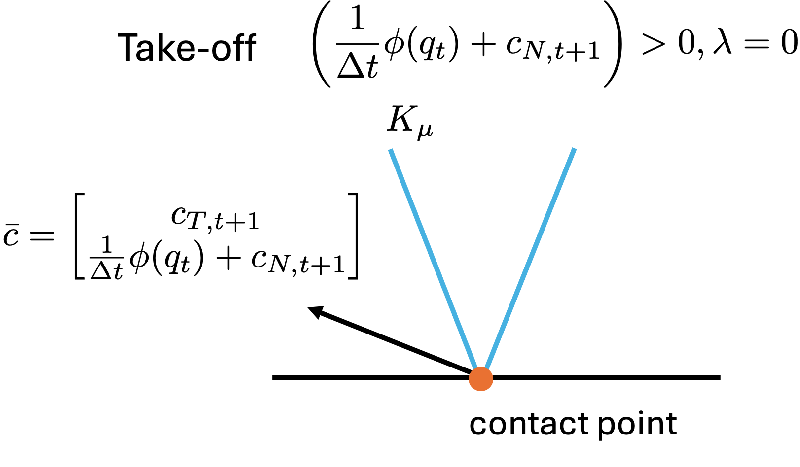

When contact is maintained, i.e., $\left( \frac{1}{\Delta t} \phi(q_{t}) + c_{N, t+1} \right) = 0$, there are two possible cases to consider: sticking and sliding.

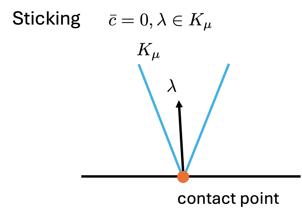
• Sticking (Static Contact)

In this situation, the tangential contact velocity is zero and the contact impulse lies in the friction cone.

• Sliding (Dynamic Contact with Friction)

In this case, according to \eqref{eq:mdp}, the tangential contact velocity is nonzero and the contact impulse reaches the boundary of the friction cone.

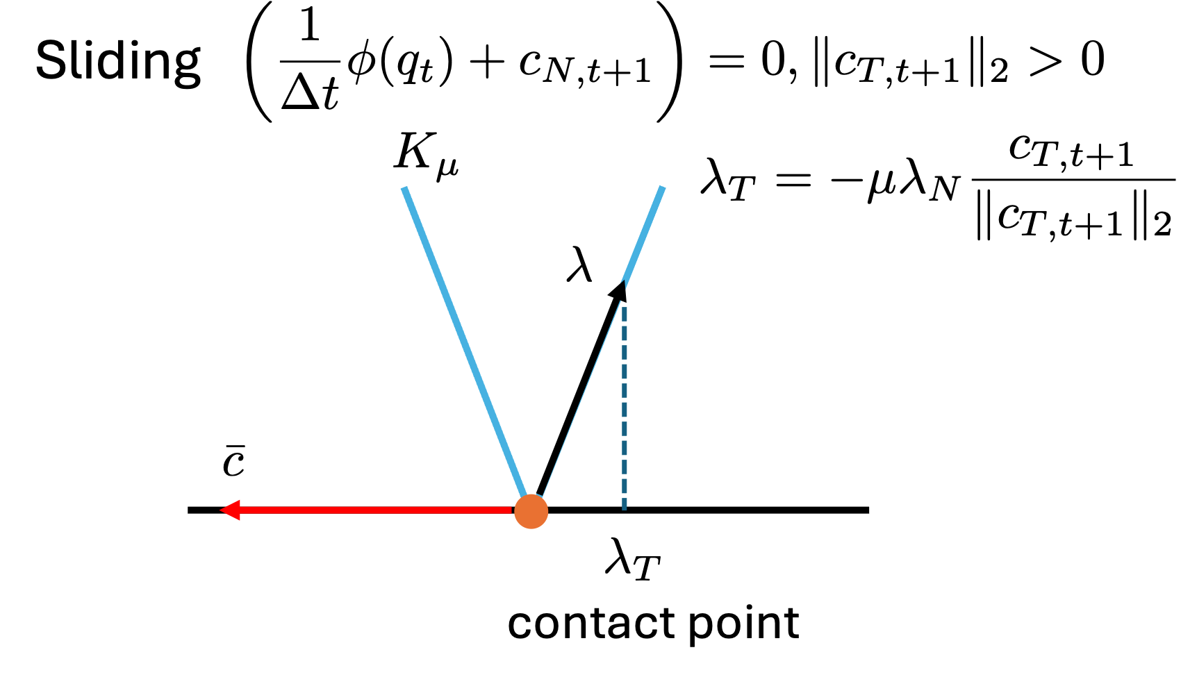
Unfortunately, we cannot obtain a compact formulation, similar to \eqref{eq:comp_constr}, using $\bar{c}_{t+1}$ and $\lambda$, since $\bar{c}_{t+1}$ is not orthogonal to $\lambda$, as shown in Figure. To get around this issue, we slightly modify $\bar{c}_{t+1}$ as follows:

\[\hat{c}_{t+1} = \bar{c}_{t+1} + \begin{bmatrix} 0 \\ \mu \Vert c_{T, t+1} \Vert_2 \end{bmatrix}.\]

Then, a compact formulation can be expressed as

\[\begin{equation} \label{eq:compact_form} K_{\mu} \ni \lambda \perp \underbrace{ \begin{bmatrix} c_{T, t+1} \\ \frac{1}{\Delta t} \phi(q_{t}) + c_{N, t+1} + \textcolor{blue}{\mu \Vert c_{T, t+1} \Vert_2} \end{bmatrix}}_{\hat{c}_{t+1}} \in K^*_{\mu}, \end{equation}\]

where $K_{\mu}^*$ denotes the dual cone of the friction cone $K_{\mu}$ defined in $\eqref{eq:f_cone}$, given by

\[\begin{equation*} \begin{aligned} K^*_{\mu} &:= \left\{ \gamma \in \mathbb{R}^3 \mid \gamma^\top \lambda \geq 0,\; \forall \lambda \in K_{\mu} \right\} \\ &= \left\{ \gamma = (\gamma_T, \gamma_N) \in \mathbb{R}^3 \mid \gamma_N \geq \mu \Vert \gamma_T \Vert_2 \right\}. \end{aligned} \end{equation*}\]

Next, we provide a visual illustration of \eqref{eq:compact_form}.

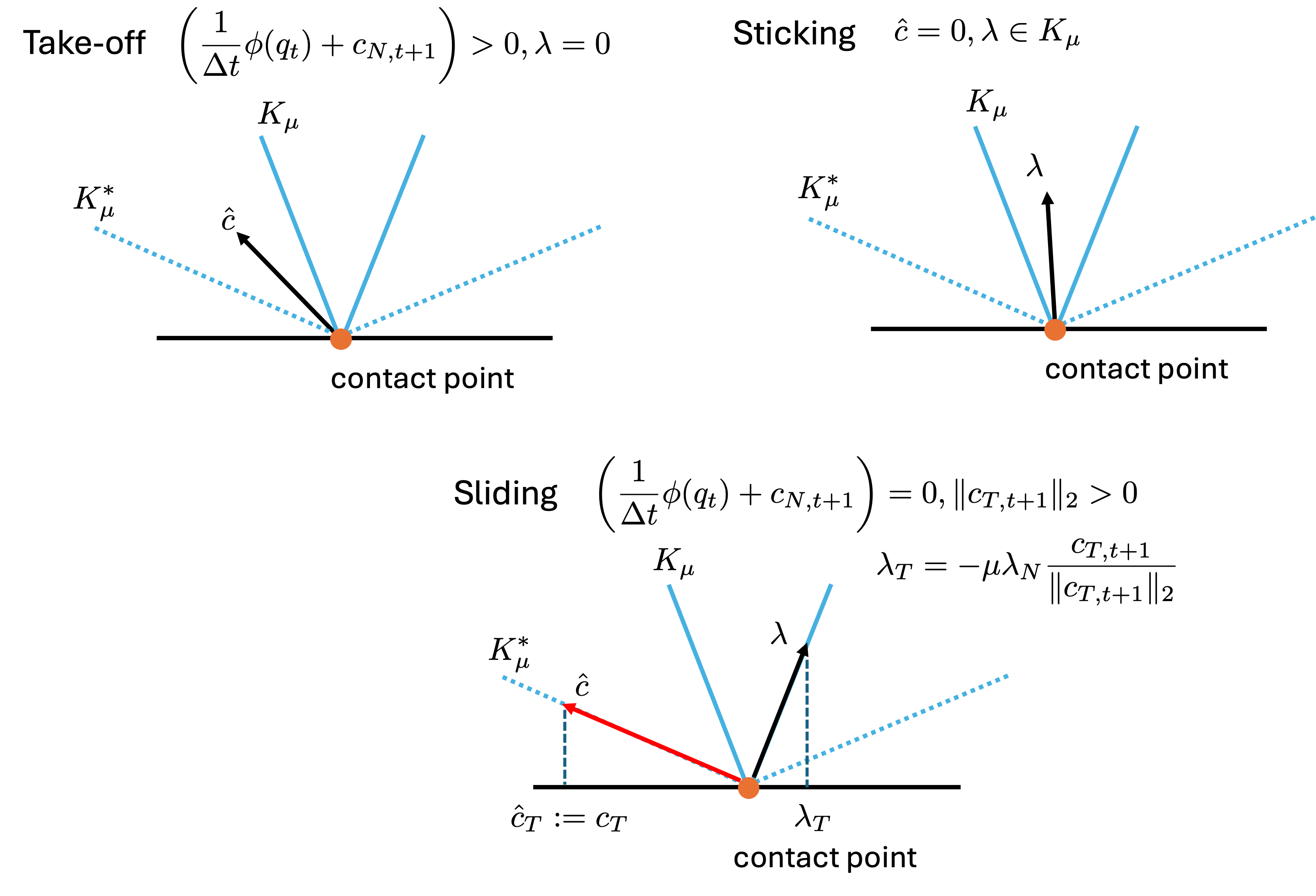
The compact formulation $\eqref{eq:compact_form}$ is a Nonlinear Complementarity Problem (NCP). Solving an NCP is challenging in general. In subsequent blog posts, we will introduce two common simplifications of this formulation: the Linear Complementarity Problem (LCP) and the Cone Complementarity Problem (CCP).

Appendix: Deriving Formulation (4) from the Signorini condition and Maximum Dissipation

This appendix derives the compact NCP formulation $\eqref{eq:compact_form}$ directly from the Signorini condition and the KKT conditions of the maximum dissipation principle. To simplify the notation, we omit the time index $t+1$ and define the discrete normal gap velocity

\[g_N := \frac{1}{\Delta t}\phi(q_t) + c_N.\]

The discretized Signorini condition is

\[\lambda_N \geq 0, \qquad g_N \geq 0, \qquad \lambda_N g_N = 0.\]

For a fixed normal impulse $\lambda_N$, the maximum dissipation principle selects the tangential impulse by solving the convex problem

\[\begin{aligned} \underset{\gamma_T \in \mathbb{R}^2}{\operatorname{minimize}} \quad & \gamma_T^\top c_T \\ \operatorname{subject\ to} \quad & \Vert \gamma_T \Vert_2 - \mu \lambda_N \leq 0. \end{aligned}\]

Let $\beta \geq 0$ be the Lagrange multiplier associated with the constraint. The corresponding Lagrangian is

\[\mathcal{L}(\gamma_T, \beta) = \gamma_T^\top c_T + \beta \left(\Vert \gamma_T \Vert_2 - \mu \lambda_N\right).\]

The associated KKT system for an optimal solution $\lambda_T$ is

\[\begin{aligned} &\Vert \lambda_T \Vert_2 \leq \mu \lambda_N, &&\text{(primal feasibility)} \\ &\beta \geq 0, &&\text{(dual feasibility)} \\ &\beta\left(\Vert \lambda_T \Vert_2 - \mu \lambda_N\right) = 0, &&\text{(complementary slackness)} \\ &0 \in c_T + \beta\,\partial \Vert \lambda_T \Vert_2, &&\text{(stationarity)}. \end{aligned}\]

The last condition uses $\in$ rather than $=$ because the Euclidean norm is not differentiable at $\lambda_T=0$. Its subdifferential is a set-valued generalization of the gradient:

\[\partial\Vert\lambda_T\Vert_2 = \begin{cases} \left\{\dfrac{\lambda_T}{\Vert\lambda_T\Vert_2}\right\}, & \lambda_T\neq0, \\[6pt] \left\{s\in\mathbb{R}^2\mid\Vert s\Vert_2\leq1\right\}, & \lambda_T=0. \end{cases}\]

When $\lambda_T\neq0$, the subdifferential contains only one vector, so the stationarity condition reduces to the usual equality

\[0=c_T+\beta\frac{\lambda_T}{\Vert\lambda_T\Vert_2}.\]

At $\lambda_T=0$, however, the subdifferential is the entire unit ball. Therefore,

\[0\in c_T+\beta\,\partial\Vert\lambda_T\Vert_2\]

means that there exists some $s\in\mathbb{R}^2$ with $\Vert s\Vert_2\leq1$ such that $0=c_T+\beta s$. This set-membership notation allows the same stationarity condition to cover both the smooth sliding case and the nonsmooth case $\lambda_T=0$.

When $\lambda_N>0$, the problem is convex and satisfies Slater’s condition, and therefore these KKT conditions are necessary and sufficient for optimality.

We now consider the degenerate case $\lambda_N=0$. The primal-feasibility condition, i.e., the first line of the KKT system, becomes

\[\Vert\lambda_T\Vert_2\leq0,\]

and therefore forces $\lambda_T=0$. The friction-cone constraint is consequently active:

\[\Vert\lambda_T\Vert_2-\mu\lambda_N=0.\]

Hence, the complementary-slackness condition is satisfied for any $\beta$. To satisfy dual feasibility and stationarity when $c_T\neq0$, choose

\[\beta=\Vert c_T\Vert_2, \qquad s=-\frac{c_T}{\Vert c_T\Vert_2} \in\left.\partial\Vert\lambda_T\Vert_2\right|_{\lambda_T=0}.\]

Here $\beta=\Vert c_T\Vert_2>0$ satisfies dual feasibility, and the choice of $s$ gives $0=c_T+\beta s$, which verifies stationarity. If $c_T=0$, choosing $\beta=0$ satisfies both conditions immediately. Thus, although Slater’s condition does not apply when $\lambda_N=0$, the unique feasible solution $\lambda_T=0$ can be verified directly against all four conditions in the same KKT system.

Next, we discuss how to solve the KKT system. If $c_T \neq 0$ and $\lambda_N > 0$, stationarity and complementary slackness give

\[\beta = \Vert c_T \Vert_2, \qquad \Vert \lambda_T \Vert_2 = \mu \lambda_N, \qquad \lambda_T = -\mu \lambda_N \frac{c_T}{\Vert c_T \Vert_2}.\]

This is the sliding solution. Substituting the expression for $\lambda_T$ above into the objective of the maximum-dissipation problem gives

\[\lambda_T^\top c_T =-\mu\lambda_N \frac{c_T^\top c_T}{\Vert c_T\Vert_2} =-\mu\lambda_N\Vert c_T\Vert_2.\]

For sticking, $c_T=0$, making both sides of this equality zero. For take-off, $\lambda_N=0$ and primal feasibility gives $\lambda_T=0$; the equality again holds. Therefore, all three contact modes satisfy

\[\lambda_T^\top c_T +\mu\lambda_N\Vert c_T\Vert_2=0.\]

Combining the KKT conditions with the discretized Signorini condition, the contact impulse and velocity must satisfy

\[\begin{cases} \lambda_N \geq 0 \\ g_N \geq 0 \\ \lambda_N g_N = 0 \\ \Vert \lambda_T \Vert_2 \leq \mu \lambda_N \\ \lambda_T^\top c_T + \mu \lambda_N \Vert c_T \Vert_2 = 0. \end{cases}\]

The first and fourth conditions are precisely the friction-cone constraint

\[\lambda=(\lambda_T,\lambda_N)\in K_\mu.\]

Next, add the two equality conditions:

\[\begin{aligned} 0 &= \underbrace{\lambda_N g_N}_{=\,0\text{ by Signorini}} + \underbrace{\lambda_T^\top c_T + \mu\lambda_N\Vert c_T\Vert_2}_{=\,0\text{ by maximum dissipation}} \\ &= \lambda_T^\top c_T + \lambda_N\left(g_N+\mu\Vert c_T\Vert_2\right). \end{aligned}\]

The last expression suggests defining

\[\hat{c} := \begin{bmatrix} c_T \\ g_N + \mu\Vert c_T\Vert_2 \end{bmatrix}.\]

With this definition, the sum of the two equalities becomes the following orthogonality condition

\[\lambda^\top\hat{c}=0.\]

It remains to locate $\hat{c}$ in the dual cone. Since $g_N\geq0$,

\[\hat{c}_N =g_N+\mu\Vert c_T\Vert_2 \geq\mu\Vert c_T\Vert_2 =\mu\Vert\hat{c}_T\Vert_2.\]

Therefore, we have $\hat{c}\in K_\mu^*$. Finally, by combining friction-cone feasibility, dual-cone feasibility, and orthogonality, we obtain

\[K_\mu\ni\lambda\perp\hat{c}\in K_\mu^*,\]

which is precisely formulation $\eqref{eq:compact_form}$.