Contact Dynamics: CCP

In the previous blog post, we introduced how to represent contact dynamics using nonlinear complementarity problems (NCPs), which are computationally challenging in general. A common approximation replaces $\hat{c}_{t+1}$ with $\bar{c}_{t+1}$, thereby dropping the nonlinear term $\mu \Vert c_{T,t+1} \Vert_2$, where $\hat{c}_{t+1}$ and $\bar{c}_{t+1}$ are

\[\begin{aligned} \bar{c}_{t+1} &:= \begin{bmatrix} c_{T,t+1} \\ \dfrac{1}{\Delta t}\phi(q_t) + c_{N,t+1} \end{bmatrix}, \\ \hat{c}_{t+1} &:= \bar{c}_{t+1} + \begin{bmatrix} 0 \\ \mu \Vert c_{T,t+1} \Vert_2 \end{bmatrix} = \begin{bmatrix} c_{T,t+1} \\ \dfrac{1}{\Delta t}\phi(q_t) + c_{N,t+1} + \mu \Vert c_{T,t+1} \Vert_2 \end{bmatrix}. \end{aligned}\]

This approximation retains the cone-complementarity structure and yields a Cone Complementarity Problem (CCP):

\[\begin{equation} \label{eq:CCP} K_{\mu} \ni \lambda \perp \bar{c}_{t+1} \in K^*_{\mu}. \end{equation}\]

A similar formulation has been used in MuJoCo, and it can be reformulated as a convex optimization problem. Before discussing the solution, we consider the potential drawbacks of this approximation by visualizing the CCP approximation.

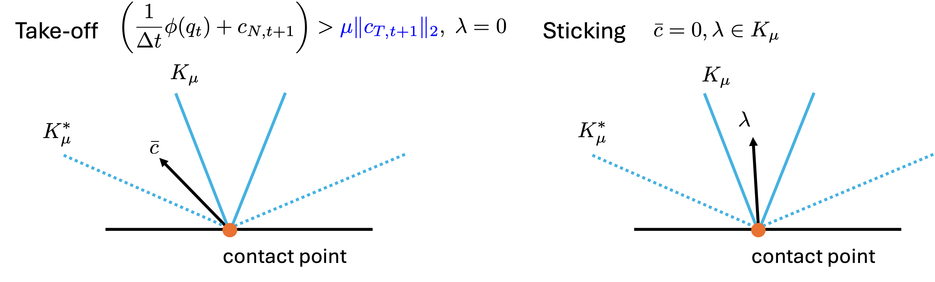
Although there is a difference in the take-off case (highlighted in blue), the CCP in \eqref{eq:CCP} can still model both situations in a reasonable way. However, an issue emerges when considering the sliding case.

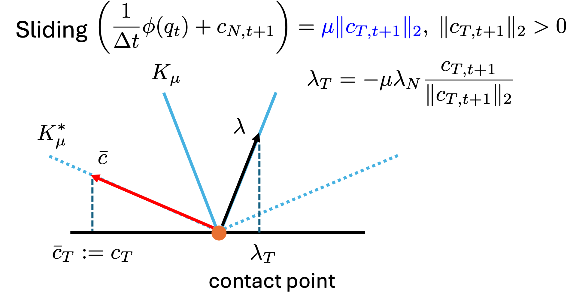
In this model, the term $\left( \frac{1}{\Delta t} \phi(q_{t}) + c_{N, t+1} \right)$ does not vanish. The normal velocity and normal impulse are both nonzero at the same time, which is physically inaccurate. For example, consider a rigid cube placed on the ground with a nonzero velocity in the x-direction. The cube should slide and gradually slow down due to friction. However, if the CCP model is used, the cube will bounce due to the nonzero normal velocity. Next, let’s see if a similar phenomenon can be observed in MuJoCo.

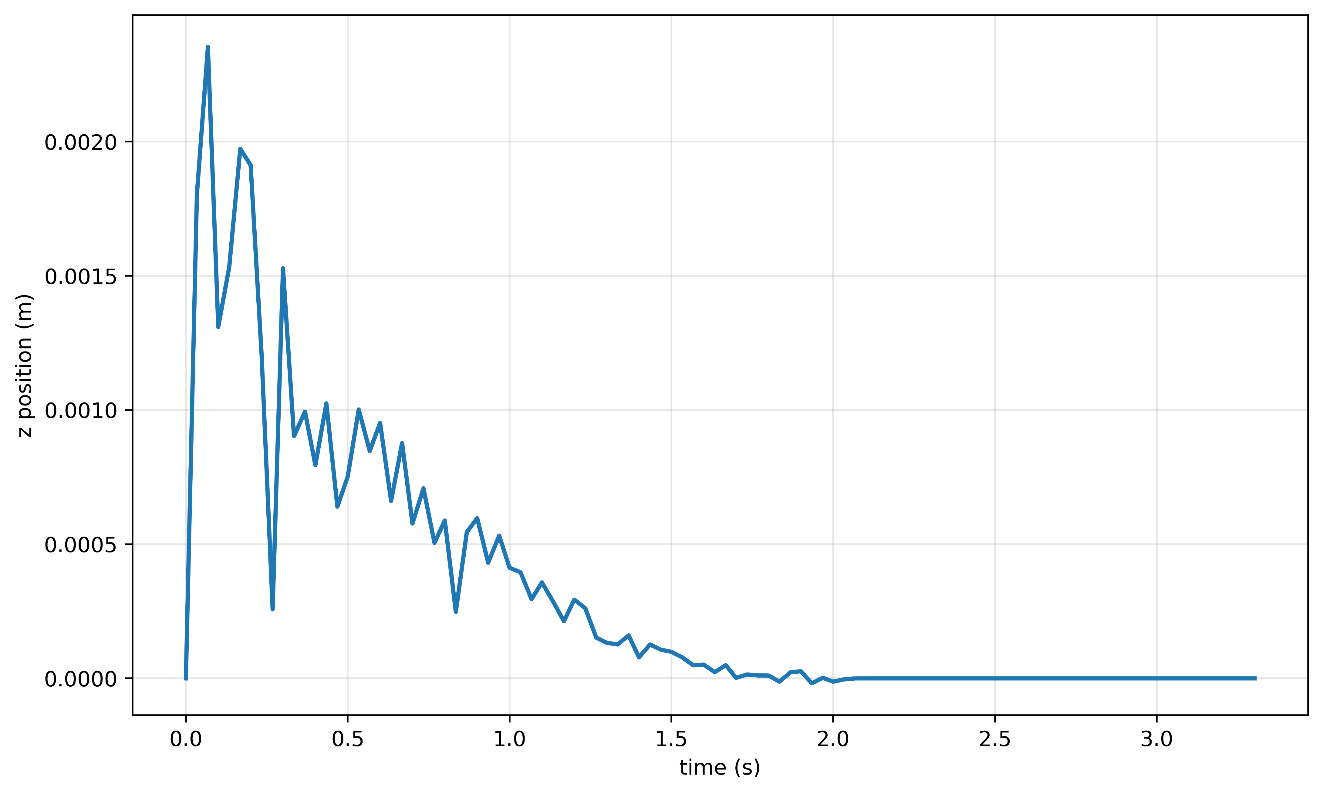
As shown in the figure above, the cube moves in the z-direction, and its displacement from the ground decreases as the tangential velocity $c_T$ diminishes. To conclude, such an artifact only emerges in the case of sliding, and its consequence can be ignored when the discretization step is small and the tangential velocity is low. In robotics applications such as grasping, locomotion, or rolling contact, the sticking mode is often of primary interest and can be precisely modeled using cone complementarity problems (CCPs).

We now delve deeper into the CCP formulation and present two types of corresponding convex optimization problems. To simplify the notation in the derivation below, we write $v := v_{t+1}$ and $c_i := c_{i,t+1}$ for the end-of-step generalized and contact velocities. We also abbreviate $M := M(q_t)$, $J := J(q_t)$, $h := h(q_t,v_t)$, and $\phi_i := \phi_i(q_t)$; the known start-of-step velocity retains the subscript in $v_t$. We begin with the CCP for the $i$-th contact:

\[\begin{equation} \label{eq:CCP_i} K_{\mu, i} \in \lambda_i \perp \bar{c}_i \in K^*_{\mu, i}, \end{equation}\]

where $K_{\mu, i}$ is the friction cone, $K_{\mu, i}^*$ is the corresponding dual cone, $\lambda_i \in \mathbb{R}^3$ represents the contact impulse, and $c_i \in \mathbb{R}^3$ is the contact velocity. We define the stabilization velocity $c_i^{\mathrm{stab}} \in \mathbb{R}^3$ as

\[c_i^{\mathrm{stab}} = \begin{bmatrix} 0 \\ 0 \\ -\frac{\phi_i}{\Delta t} \end{bmatrix},\]

so that the CCP contact-constraint vector is

\[\bar{c}_i := c_i - c_i^{\mathrm{stab}}.\]

Here, $\Delta t$ is the discretization step. Let $N_c$ denote the number of contacts. Next, we derive two optimization problems whose KKT conditions are equivalent to the problem in \eqref{eq:CCP_i}.

Optimization on the dual

We aim to formulate an optimization problem in terms of the contact impulse $\lambda$, which serves as a dual variable in constrained multibody dynamics. To achieve this, we first replace the contact velocity $c$ with the contact impulse $\lambda$. To achieve this, we revisit the discretized multibody dynamics:

\[M(v - v_t) = \Delta t\left(\tau_t - h\right) + J^\top \boldsymbol{\lambda},\]

By rearranging the equation, we derive the expression for $v$ in terms of $\lambda$:

\[\begin{align} M v &= J^\top \boldsymbol{\lambda} + M v_t + \Delta t\left(\tau_t - h \right) \label{eq:dynamics} \\ v &= M^{-1} J^\top \boldsymbol{\lambda} + \underbrace{v_t + M^{-1} \Delta t\left(\tau_t - h \right)}_{v^f} \nonumber \end{align}\]

where the inertia matrix $M$ is always invertible, and $v^f$ is the free motion velocity that the system would have in the absence of contact constraints. We then compute the contact velocity by multiplying both sides by $J$:

\[\begin{equation} \label{eq:c_lambda} \begin{aligned} \boldsymbol{c} &= J v \\ &= J M^{-1} J^\top \boldsymbol{\lambda} + J v^f \\ &= G \boldsymbol{\lambda} + J v^f, \end{aligned} \end{equation}\]

Here, $\boldsymbol{c} = [c_1^\top, \dots, c_{N_c}^\top]^\top$ is the stacked vector of end-of-step contact velocities, and $G := J M^{-1} J^\top$ is the so-called Delassus matrix. Substituting \eqref{eq:c_lambda} into \eqref{eq:CCP_i}, we rewrite the CCP as

\[\begin{equation} \label{eq:CCP_dual} \begin{aligned} G \boldsymbol{\lambda} + g &= \bar{\boldsymbol{c}} = \boldsymbol{c} - \boldsymbol{c}^{\mathrm{stab}} \\ \lambda_i &\in K_{\mu, i},\; i = 1, \dots, N_c \\ \bar{c}_i &\in K_{\mu, i}^*,\; i = 1, \dots, N_c \\ \boldsymbol{\lambda}^\top \bar{\boldsymbol{c}} &= 0, \end{aligned} \end{equation}\]

where $\boldsymbol{c}^{\mathrm{stab}} = [(c_1^{\mathrm{stab}})^\top, \dots, (c_{N_c}^{\mathrm{stab}})^\top]^\top$ and $g = J v^f - \boldsymbol{c}^{\mathrm{stab}}$. In fact, the conditions above can be viewed as the KKT conditions of the following optimization problems in terms of $\lambda$:

\[\begin{aligned} \min_{\boldsymbol{\lambda}}\; &\dfrac{1}{2} \boldsymbol{\lambda}^\top G \boldsymbol{\lambda} + g^\top \boldsymbol{\lambda} \\ \text{s.t.}\; & \boldsymbol{\lambda} \in \mathcal{K} := K_{\mu, 1} \times \dots \times K_{\mu, N_c}. \end{aligned}\]

The Lagrangian function is given by

\[\mathcal{L}(\boldsymbol{\lambda}, \boldsymbol{y}) = \dfrac{1}{2} \boldsymbol{\lambda}^\top G \boldsymbol{\lambda} + g^\top \boldsymbol{\lambda} - \boldsymbol{y}^\top \boldsymbol{\lambda},\]

where $\boldsymbol{y}$ is the Lagrange multiplier vector. The corresponding KKT conditions are then

\[\begin{aligned} G \boldsymbol{\lambda} + g &= \boldsymbol{y} &&\text{(stationarity)} \\ \boldsymbol{\lambda} &\in \mathcal{K} &&\text{(primal feasibility)} \\ \boldsymbol{y} &\in \mathcal{K}^* &&\text{(dual feasibility)} \\ \boldsymbol{y}^\top \boldsymbol{\lambda} &= 0 &&\text{(complementary slackness)} \end{aligned}\]

This formulation is equivalent to \eqref{eq:CCP_dual} when $\bar{\boldsymbol{c}} = \boldsymbol{c} - \boldsymbol{c}^{\mathrm{stab}}$ is interpreted as the Lagrange multiplier vector.

Optimization on the primal

We now introduce an alternative optimization problem, where the decision variable is the generalized velocity $v$.

From \eqref{eq:dynamics}, we have

\[M v = J^\top \boldsymbol{\lambda} + M v^f.\]

We then reformulate \eqref{eq:CCP_i} as

\[\begin{equation} \begin{aligned} M (v - v^f) - J^\top \boldsymbol{\lambda} &= 0 &&\text{(stationarity)} \\ J v - \boldsymbol{c}^{\mathrm{stab}} &\in \mathcal{K}^* &&\text{(primal feasibility)} \\ \boldsymbol{\lambda} &\in \mathcal{K} &&\text{(dual feasibility)} \\ \boldsymbol{\lambda}^\top (J v - \boldsymbol{c}^{\mathrm{stab}}) &= 0 &&\text{(complementary slackness)} \end{aligned} \end{equation}\]

Again, the conditions above correspond to a convex optimization problem:

\[\begin{aligned} \min_{v}\; &\dfrac{1}{2} (v - v^f)^\top M (v - v^f) \\ \text{s.t.}\; & J v - \boldsymbol{c}^{\mathrm{stab}} \in \mathcal{K}^*. \end{aligned}\]

Its Lagrangian function is given by

\[\mathcal{L}(v, \boldsymbol{\lambda}) = \dfrac{1}{2} (v - v^f)^\top M (v - v^f) - \boldsymbol{\lambda}^\top (J v - \boldsymbol{c}^{\mathrm{stab}}),\]

where the vector of contact impulses $\boldsymbol{\lambda}$ coincides with the dual variable of the optimization problem.